Appendix N — PART C — NE’ER THE TWAIN SHALL MEET?
PART C: NE’ER THE TWAIN SHALL MEET?
~ 19 min reading
1. Introduction
Well, the twain may meet—but there’s often a serious problem when they do: neither can understand what the other is talking about! The “twain” to whom I am referring are students from what we might call the Deming/Shewhart school of Statistics on the one hand and from the “conventional” or “traditional” or “mathematical” school of Statistics on the other. As I said as early as Day 1 page 6, and repeated here in the Introduction on page 2:
“Over the nearly 20 years of my seminars on Dr Deming’s teaching I rarely suffered from any ‘difficult’ delegates. The few that I had could be divided into two types. One type were very senior managers; the other type were those with some qualification in Statistics.”
On page 2 I then pointed out that
“… the latter were often the more difficult type. That may sound rather flippant, but it isn’t. It can be very serious. If it happens to you then I want to help you to deal with it. For you may not have any qualification in Statistics. So are the people in your organisation likely to believe you or the one who is qualified in the subject?”.
For example, the “conventional” student has been taught that both the theory and “validity” of control charts depend upon traditional Mathematical Statistical fodder such as probability theory, the normal distribution, the Central Limit Theorem, and hypothesis testing. The Deming/Shewhart student may never even have heard of such things because, truth to tell, neither the “validity” nor even the basic ideas behind control-chart methodology depend on any of them—at least, that is, according to both Dr Walter Shewhart (who, as you know, was the subject’s creator) and his famous protégé, Dr W Edwards Deming (and, by now, you know quite a lot about him as well!). I’d say they were both fairly safe sources of wisdom. However, if you are interested in what those things are about, you will find some explanation and discussion on them in Part D of these Optional Extras—and that will be useful if you ever become one of the twain that do meet! Why? Well, let’s see.
You, the Deming/Shewhart student, might well like to convince the conventional Statistics student that those supposed mathematical underpinnings are irrelevant. But how can you, if you know not what they are, let alone why the conventional student deems them to be so essential? Yet you almost certainly need to be able to communicate such arguments, else your organisation will continue to be held back by misconceptions taught to them by the statistical “expert”, misconceptions that are very likely to result in overrestrictive use of control charts and often fear of their use. As Dr Deming pointedly expressed it (Out of the Crisis page 286[335]), the mathematical concepts mentioned above “are misleading and derail effective study and use of control charts”. I most certainly could not have expressed it better myself. So some of the material that follows attempts to enable you (a) to understand how the conventional statistician thinks, and why he thinks that way, and (b) to thus be able to communicate with him, and then (c) to have at least a sporting chance of helping him see the error of his ways.
One big problem that exists between the two schools is that there are likely to be incompatibilities of perceived purpose, and therefore of use and interpretation, of control charts. The Deming/Shewhart student recognises control charts as a valuable guide to appropriate action for improvement. The conventional student usually regards them merely as a monitoring device to provide an early warning of something going wrong, so as to trigger timely corrective action. But that is not improvement—it is, at best, maintenance of the status quo.
That is clearly a matter touching upon the very management philosophy and approach of the organisation in which the control charts are being used—thus it is strongly related to the main material of this course. The concentration here in this optional material is largely restricted to merely technical issues. But students from the two schools often find that, even on technical matters, they still cannot understand each other.
The clear rejection by both Shewhart and Deming of the relevance of the conventional statistician’s “lifeblood” of probability calculations and normal distributions in this context have already been evidenced by quotations from both of them that you have seen in the main text. But they surely bear repeating here.
Firstly, there was the extract from Out of the Crisis page 286[pages 334–335] that I have just mentioned, and I make no apology for repeating part of the final sentence:
“It would … be wrong to attach any particular figure to the probability that a statistical signal for detection of a special cause could be wrong, or that the chart could fail to send a signal when a special cause exists. The reason is that no process, except in artificial demonstrations by use of random numbers, is steady, unwavering.
It is true that some books on the statistical control of quality and many training manuals for teaching control charts show a graph of the normal curve and proportions of area thereunder. Such tables and charts are misleading and derail effective study and use of control charts.”
Then there was this extract from page 12 of Shewhart’s 1939 book:
“Some of the earliest attempts to characterise a state of statistical control were inspired by the belief that there existed a special form of frequency function f and it was early argued that the normal law characterised such a state. When the normal law was found to be inadequate, then generalised functional forms were tried. Today, however, all hopes of finding a unique functional form f are blasted.”
And finally there was this passionate language from Deming when he was speaking to some senior executives in France in 1989 (recorded in Profound Knowledge, BDA Booklet A6 page 4 and recently already mentioned here on page 20 of these Optional Extras):
“How can we aim for minimum economic loss? It is nothing to do with probabilities of the two kinds of mistakes. No, no, no, no: not at all. What we need is an operational definition of when to look for a special cause, and when not to. That is, a rule which guides us when to search in order to identify and remove a special cause, and when not to. It is not a matter of probability. It is nothing at all to do with how many errors we make on average in 500 trials or 1,000 trials. No, no, no—it can’t be done that way. We need an operational definition of when to act, and which way to act. Shewhart provided us with a communicable operational definition: the control chart using 3σ-limits. Shewhart contrived and published the rules in 1924—65 years ago. Nobody has done a better job since.”
2. The essence of the argument
Two types of “statistical studies”
Assuming you do not have much or any background in conventional Statistics, this section will (like the first section) contain some words, terms and phrases with which you are not familiar. But please read it nonetheless! My purpose here is to provide a broad introductory description of all of the rest of this optional extra material so that you can get an advance sense of the shape of things to come. This includes (on page 33) a typical syllabus for an introductory course on conventional Statistics which obviously will indeed include some terms with which you are unfamiliar. But, after reading these current two pages, you will have a good idea of why I am introducing them to you. They are mostly “part and parcel” of what the conventional statistician is familiar with, and so then you will have a chance of discussing things with him. That will be even more the case if you undertake the “crash-course in conventional Statistics!” that I offer you in Part D.
But even the conventional statistician will probably not be familiar with some or all of what I shall now introduce—so you’re on a level playing-field for the time being! At least, that was my experience with what follows. Maybe a couple of years before I first met Dr Deming, I tried to read some of what he had written about the subject of Statistics. And almost immediately I was faced with terms such as “analytic studies”, “enumerative studies” and “frames”. All totally new to me.
Now, at that time, I had already been a Lecturer in Statistics in the University of Nottingham’s Department of Mathematics for over 15 years. So I suppose I had already become somewhat set in my ways and in my understanding. For it seemed from what I was reading that Deming was claiming all I had so far learned and had therefore so far been teaching others, was “merely” concerned with “enumerative” studies—whereas what was really needed in order to be useful in the real world was “analytic” studies. Surely that couldn’t be right, could it?
But a lot of other stuff that Deming had written did appeal to me, so I rather set aside that business about the two types of statistical studies and read about other things instead. Nevertheless, some time later when the British Deming Association began its work, one of the first things I did was to set up a study group to examine Deming’s writings about Statistics to see if that group could shed some light on those puzzling matters. I was extremely fortunate to have the late Professor David Kerridge as leader of that study group, and light eventually began to dawn under his patient and wise guidance. David became a great supporter and helper and friend in the years that followed.
Again assuming that you do not have much background in conventional Statistics, you probably won’t have the mental blocks that I had and will therefore be able to get the gist of what Deming was writing about much more quickly than I did.
What do dictionaries tell us about those puzzling words? Actually, I discovered that neither dictionaries on the internet nor in print seem very helpful with the adjective “enumerative”. All I could find was either the noun “enumeration” or the verb “enumerate” with “enumerative adj” then appearing merely as an appendage without definition. The verb “enumerate” is typically described as “To count off or name one by one; list” and the noun “enumeration” as “The act of enumerating” or “A detailed list of items”. Is that really all I had been teaching all those years?!
Maybe I’d have better luck with “analytic”. A well-known dictionary on the internet produces: “Generally speaking, ‘analytic’ refers to ‘having the ability to analyse’ or ‘division into elements or principles’.” OK: maybe that makes a bit of sense. How about my favourite hard-copy dictionary—what did I find there? “Of, pertaining to, or based on analysis; showing an ability to analyse and reason from a perception of the parts and interrelationships of a subject; skilled in analysis.” Hmm, I found a glimmering there, but not a lot.
How about “enumerative study” or “analytic study”? No: I drew a blank on both of those.
So I’d better try some brief explanations in my own words! “Analytic studies” are indeed what we have been involved with, particularly in the early days of 12 Days to Deming, primarily enabled by the use of control charts. Let me try a description in just a single sentence: The purpose of analytic studies is to enhance knowledge and understanding of processes, for prediction into the future, and to provide guidance for improvement. You will observe that we could just as well replace “analytic studies” by “control charts” in that sentence. Looking back to the early years of my career-life, I must indeed confess that that sentence does not describe what I was then teaching. I had actually come across a version of control charts in a book quite early on while teaching in America, and thought the topic interesting enough to devote, say, half of a 50-minute lecture to it in the introductory Statistics course that I gave back here in the UK, but I certainly cannot claim that that sentence describes what I taught during those few minutes. (No, I shall not embarrass myself by describing to you what I did cover in them!)
How about a brief explanation of “enumerative studies” in my own words? As we shall see later, an introductory course on conventional Statistics often begins by talking about drawing a sample (or preferably a “random sample”) from a “population”. A “population” is some collection of “things”—possibly people but often not. In the Red Beads Experiment, the population is a collection of 4,000 beads. A “sample” from the population is, of course, a sample from that collection of those “things” from the population—we are familiar with samples consisting of 50 beads obtained using the “paddle”. If the term “random sample” is used, what does that imply? It actually implies something very specific: namely, that each and every possible sample (of the specified size) is equally likely to be drawn as any other. Using the sample, the output from an “enumerative study” is then an attempted description of what is in that population—or, rather, in that part of the population which is available for sampling, and that’s what Deming meant by the word “frame”. A census is a good example of an enumerative study using an extremely large (though not random) sample.
Note that simply attempting to describe what is in the population (or frame) does not include any intent to explain why the population (frame) contains what it does nor what anything related to it might become or deliver in the future. As Deming would say, it contains no “temporal spread”. So in an enumerative study, there is no reason to consider matters such as whether or not a state of statistical control exists—indeed, the times at which the data are taken are often not even noted—whereas, of course, that is top priority in analytic studies. As I understand it, this is the essential difference between those two types of statistical studies—and, as I believe you will appreciate, that’s a big difference. There may well be more, but at least I hope this will give you a reasonable start if you ever do decide to delve into such matters.
If books and courses on Statistics were to make clear—maybe not using the same terms, but at least indicating the purpose and limitations—that what they include is designed only for enumerative rather than for analytic studies, presumably they would not do much harm. However, if one looks at the examples illustrated in, say, chapters on histograms in introductory Statistics texts, even in the more “practical” ones, it is often the case that they are actually involved not with “populations” but with processes, i.e. with their data being generated over time and with a strong likelihood that time-dependence is important. Thus, not only are the purpose and limitations of enumerative studies not made clear—it would appear that they are not even recognised by many authors and teachers.
A typical syllabus for an introductory Statistics course
To help you understand something of the conventional statistician’s mindset, Part D of these Optional Extras will introduce you to some content of a typical introductory Statistics course. But, to prepare you for that pleasure, here is a possible syllabus for such a course. Again it will, of course, contain some terms that are unfamiliar to you—but then that is likely to be true of a syllabus for a course on any topic with which you are not already familiar.
- Summarising “raw data” through pictures such as histograms and the calculation of “sample statistics” such as the sample mean X̄ and the sample standard deviation s and/or the sample variance s² [a “sample statistic” is anything which can be computed from the data in the sample].
- Probability, particularly as the long-term proportion of occurrences of an event and using symmetry considerations (as with coins, dice and playing cards).
- The natural link between the above two topics, i.e. that if one takes an ever-larger random sample from a population then the corresponding histogram (appropriately scaled) gets ever-closer to a similar pictorial representation of the probabilities of the possible outcomes—thus leading to the ideas of the “true mean” μ and the “true standard deviation” σ of a probability distribution being respectively the long-term values of X̄ and s as the sample size n → ∞ (“tends to infinity”).
- Discrete and continuous probability distributions: particularly the binomial and normal distribution respectively.
- Properties of the normal distribution, including the Central Limit Theorem.
- Statistical inference: in particular, confidence intervals and hypothesis tests (tests of significance), and how assumptions of normality and/or the use of the Central Limit Theorem enable these to be placed on an appealing mathematical footing.
There; that’s going to be fun, isn’t it?
The conventional statistician’s view of control charts, …
Here is an abbreviated version of Deming’s second quotation on page 30:
“How can we aim for minimum economic loss? It is nothing to do with probabilities of the two kinds of mistakes. No, no, no, no: not at all. … It is not a matter of probability. It is nothing at all to do with how many errors we make on average in 500 trials or 1,000 trials. No, no, no—it can’t be done that way.”
As you will see later, Deming was alluding here to the conventional statistician attempting to treat control charts as if they were hypothesis tests. A hypothesis test results in the rejection or acceptance of a so-called “null hypothesis” H₀. This decision is made according respectively to whether an appropriate sample statistic, the “test statistic”, lies inside or outside some region of values defined by one or two “critical values”: this region is therefore called the “critical region”. Moreover, the “significance level” of the test is defined to be the probability of the test statistic wrongly rejecting H₀, i.e. rejecting H₀ (because its value falls inside the critical region) when H₀ is in fact true. So that’s the direct connection with what Deming was talking about above. Assumptions about the data being normally distributed, or equivalently the Central Limit Theorem, allow particularly easy and convenient derivation of the critical value(s) for any desired significance level.
If the conventional statistician, trained in this way, subsequently comes across a control chart—by far the most important tool for an analytic study—it is rather easy to see why he is immediately inclined to regard it as a kind of glorified hypothesis test with H₀ representing “in statistical control”, and why he thinks that normality has such an important part to play. But, as we have seen, the traditional Statistics course such as that whose syllabus is summarised above is based upon foundations only pertaining to enumerative studies—in particular, ignoring any questions about behaviour possibly changing over time. (There are a few areas in conventional Statistics that study behaviour changing over time in some specified well-defined manner. But that’s a very different matter, and actually probabilities and the normal distribution again often dominate the theory in such areas.) The conventional statistician’s interpretation of a control chart as a glorified hypothesis test is thus wholly without foundation in practice. As a matter of fact, even in enumerative studies, aspects of hypothesis testing stand on rather thin ice because, in most practical applications, H₀ is never, or almost never, true! So I’m rather glad that “in statistical control” is not an appropriate H₀!
The conventional statistician will hardly give a friendly hearing to the suggestion that the foundations upon which he has built his beliefs, career and reputation might be inappropriate in the “real world” as opposed to in the Mathematics classroom. So, is there anything that can be done? Yes, fortunately and remarkably, there is.
But, before that, it is worth making the intriguing and salutary point that Shewhart himself started out thinking that the subject could be developed from the conventional Statistics viewpoint. What is often referred to as “the very first control chart” (pictured below, dating from 1924) shows some guidelines placed at just one standard deviation either side of the Central Line, with the indication “68% p” written against them. That probability, expressed as a percentage, is derived from the normal distribution, as you will be able to confirm when you reach page 49.
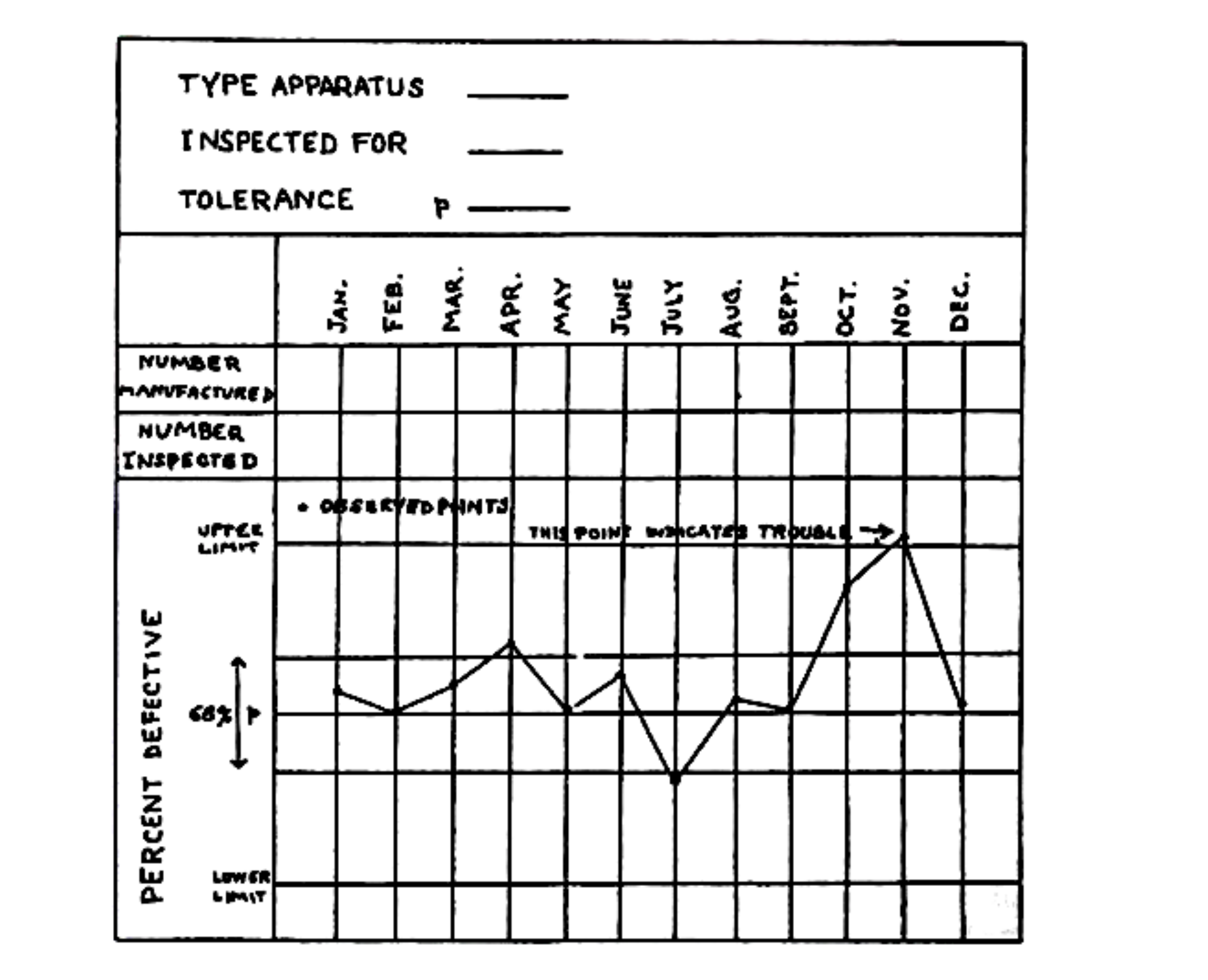
Yet, despite this, Shewhart was open-minded enough to eventually see the error of this mode of thinking. His statement on page 30 (sandwiched between the two quotations from Dr Deming) was clearly autobiographical!
… and what can be done about it
Substantially, the conventional statistician’s case for requiring normality to make control charts and their control limits “valid” exists on two main fronts. Such a statistician believes that normality is needed:
- because control-chart constants that are used in computation of control limits, such as the 2.66 with which we became familiar on Day 3, are derived from normal distribution theory (as indeed they are); and
- so that a probability interpretation can be given to control limits: specifically, the claim is often made that, under normality, there is a probability of 0.0027 (i.e. 0.27%) that any particular data-point falls outside Shewhart’s 3σ-limits (note that 0.27% = 2 × 0.135% when you look at page 49) if the process is in statistical control.
Now again, any acceptance of Shewhart’s and Deming’s teachings immediately leads to the denial of the conventional statistician’s claims in both of these respects. The “fortunate and remarkable” facts alluded to on the previous page are however that, even if we ignore what Shewhart and Deming said about both normality and probability interpretations (recall, in particular, page 30), the above claims are still demonstrably wrong! In other words, we are able to wade right into the conventional statistician’s camp, onto ground which both Shewhart and Deming believed to be without foundation yet which the conventional statistician needs to have faith in (for all that he has learned is built upon it), and to talk to him in language which he both understands and accepts (even if we don’t), and to still produce evidence which disproves his beliefs!!
That evidence is demonstrated in Part E on pages 65–70.